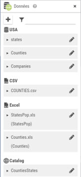
The data panel shows the available datasets list for the actual documents (queries of the actual document and imported files).
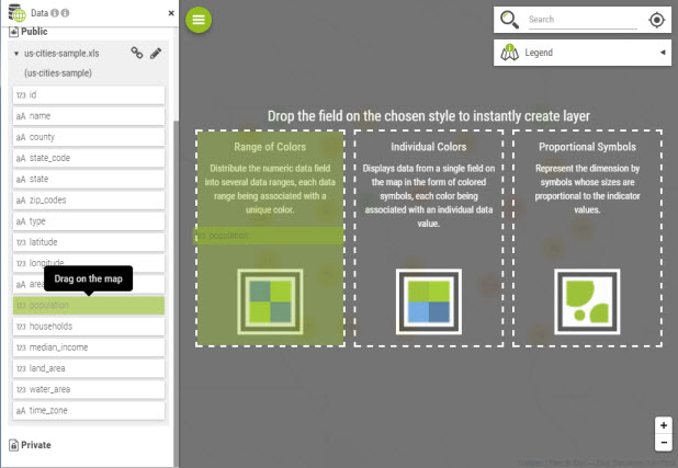
Each dataset can be unfolded and thematic layers can added to the map using a single drag and drop:
|
The right can vary according to the dataset. When a user is not allowed to edit a dataset, then creation of thematics by drag and drop is forbidden |
Intermediate
users and above have access to the  button to
add some content. There are two possibilities:
button to
add some content. There are two possibilities:
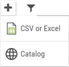
a CSV or Excel dataset:
One can choose an Excel or CSV file from the own system or from a resource on the network. When importing an Excel file type XLSX the size limit is 1MB.
a layer from the catalog of geographic data:
The data contained in the layer will be imported.
|
The CSV / Excel import is available as an extension and the feature is controlled by the product license. |
|
The catalog represents the list of vector map services declared in the administration console. It also include the territory projects that have been published. |
|
One can copy/paste a Galigeo eXperience custom element, or a WebI document containing a custom element, however the imported datasets and the created territory management project will not be copied. |
The matrix bellow sums up all the possibilities for the rights:
User type |
Dataset privacy |
Is Owner |
Can View ? |
Is Editable ? |
End user |
Public |
|
YES |
NO |
End User |
Private |
|
NO |
NO |
Intermediate User |
Private |
YES |
OK |
OK |
Intermediate User |
Private |
NO |
NO |
OK |
Intermediate User |
Public |
NO |
YES |
NO |
Author / Designer |
Public |
YES |
YES |
YES |
Author / Designer |
Public |
NO |
YES |
YES |
Author / Designer |
Private |
YES |
YES |
YES |
Author / Designer |
Private |
NO |
NO |
NO |
As soon as a data is imported, the data wizard is opened.
The
data wizard can be opened anytime later by clicking on  .
.
The data preview displays a subset of the current dataset. The panel allows to:
Rename the dataset
Delete the dataset
Update the dataset (this is used to update the data, however make sure to re-import a file that has exactly the same structure). This button is not available at the initial import of the dataset.
Export the dataset as CSV, GeoJson or Shape file
Make the dataset private/public
Depending of the dataset type, some of these controls can be missing. For example, catalog dataset cannot be re-imported since it is linked to an existing catalog layer. In some cases, a user might not be authorized to edit the dataset ; in which case most controls are disabled.
|
The file used for update has to have exactly the same structure (number and names of columns) and has to be the same type as the original file used when the dataset was imported. |
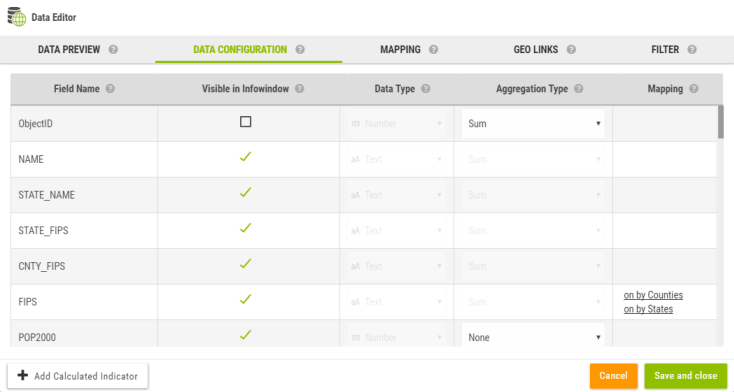
The data configuration is used to set the attributes of each individual columns. In that panel, you can
Rename a column
Make it visible or not in the infowindow
Force the data type (available only for CSV files)
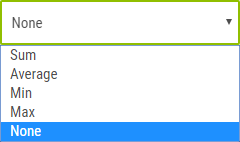
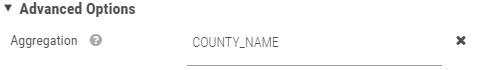
Set the aggregation operator. This operator is applied anytime the map needs to aggregate the data.
|
For example an indicator can be define by zipcode and by year in the original dataset. In that case, the indicator will be displayed by zipcode on the map and the indicators will by aggregated by year. |
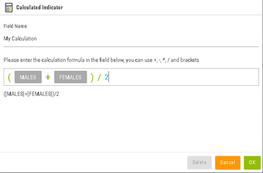
Add a calculated indicator
 in order to add new columns
calculated using another set of indicators.
in order to add new columns
calculated using another set of indicators.
List of aggregation operators:
|
|
|
Galigeo application is using field position in the query or data source and can be impacted by any modification of the query:
|
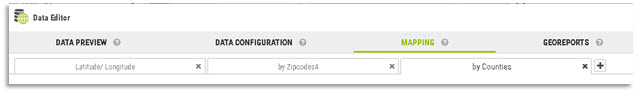
The mapping tab is used to defined how the current dataset is transformed into a geographic dataset.
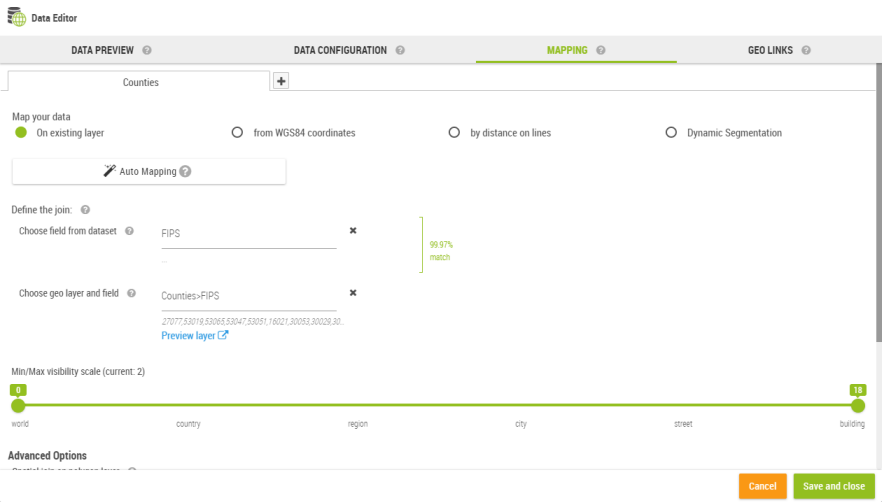
The product supports three main types of mapping:
Join on a geographic layer
XY coordinates
Native geometry (when the original dataset is already spatial, ex: catalog dataset)
This type of mapping is literally a join between two dataset:
The dataset being edited
A geographic layer which is technically another dataset with a geometry column
The user must select a valid join key on both sides in order to get the mapping to work.
|
Example: the zipcode column of a CSV with the zipcode column of a catalog layer. |
The list of catalog layers displays all known geographic layers used in the application.
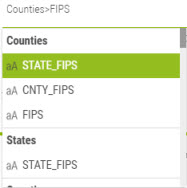
Finding the correct match can be difficult especially when the user is not familiar with the notion of geographic layer. To simplify the task, Galigeo provides an auto-mapping feature to automatize the process:

In most cases, this feature will find automatically the best possible mapping.
The XY mapping type is used when the dataset contains natively some X/Y columns representing the longitude/latitude coordinates of points. The XY values must be specified.
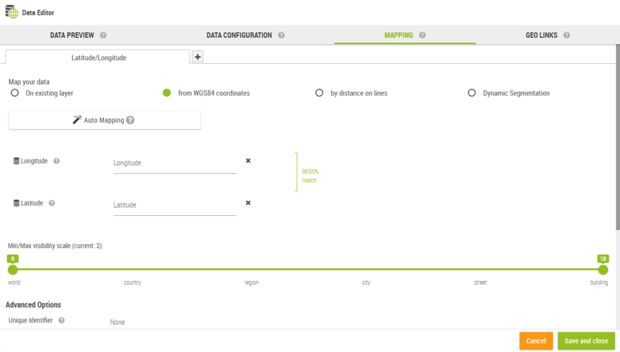
|
Example: The dataset represents a list of stores with two columns longitude and latitude. These columns contain the GPS coordinate of each stores in degree. |
Optionally, a unique Id can be specified with this type of mapping:
The dynamic segmentation mapping is available in the form of an optional module.
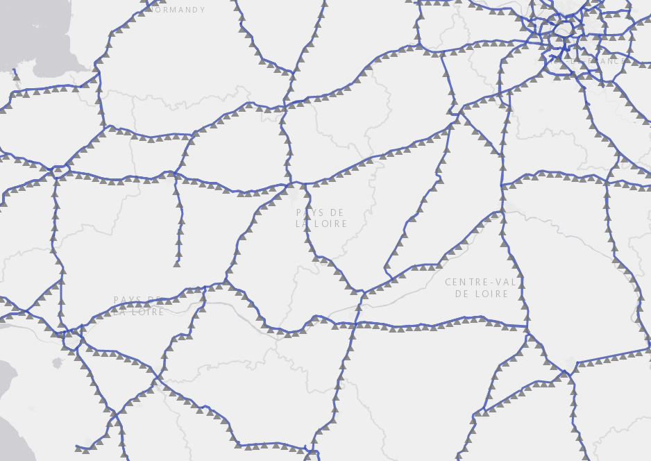
The dynamic segmentation is based on a linear data network (networks of roads, railroads, pipes, etc.) and allows the representation of segments placed between two reference points.
This implies that we have a reference points system associated to a network. For instance the milestones on roads. The available networks list is defined on Galigeo Manager.
The represented data on the map are expressed in the form PR + Abscissa, i.e. a point on the map is identified by a reference point and by a distance in meters.
Example: 50PR49D + 650 correspond to the point placed at 650 meters from the milestone 50PR49D.
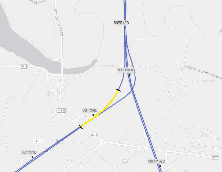
On the above example, the data received by Galigeo are expressed in the following manner:
Axis |
Start PR |
Start Abscissa |
End PR |
End Abscissa |
Other Indicators … |
A86 |
50PR49D |
650 |
50PR50D |
200 |
|
We find the same parameters on the configuration interface of the MAPPING tab:
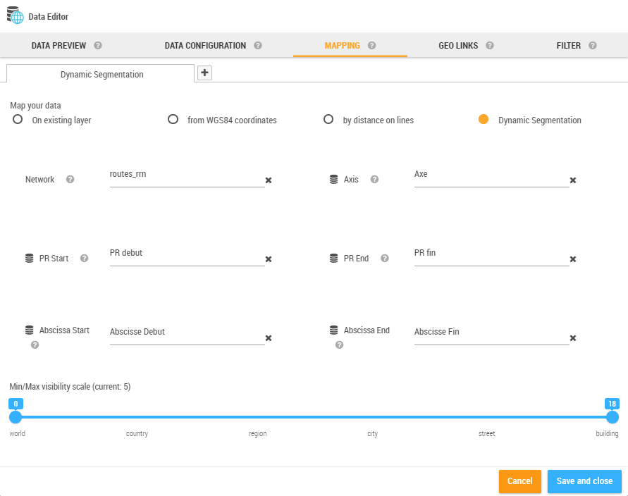
|
The Auto Mapping is not available for this type of mapping. |
Network Management
The management of available networks is done from the Galigeo Manager > Dynamic Segmentation.
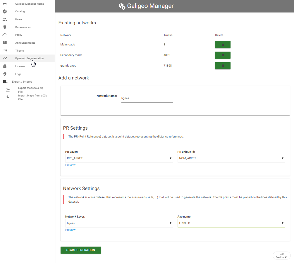
At the top of the page are listed the existent networks and allows the deleting of them if needed.
The sections “PR Settings” and “Network Settings” allow the selecting of data to use for the generation of a new network.
For the reference point one has to select from the catalog a points layer as well as the attribute that will serve to name the PRs.
For the lines, one has to select the layer representing the associated axes associated to each PR.
It is important that the two selected layers are in a relationship one to the other in order to give the expected result.
The “Start Generation” button starts the creation of the network. This operation may take several minutes according to the data to process. For this reason Galigeo is blocking the parallel creation of two networks (even from two simultaneous users).
Auto-mapping
The auto-mapping feature is available for all mapping types.
The auto-mapping use a smart algorithm to detect automatically how to represent a dataset on the map. In most cases, the auto-mapping is able to find itself the best representation.
It is possible the auto-mapping fails and here are the main reasons for it:
The catalog does not have an appropriate layer to represent the dataset. If that’s the case, you need to register a new layer to the catalog (this is done once for all users).
The data types are not correct. For example a zipcode column might be defined as a number but is defined as a string in the geographic layer. In that case, you need to change the data type in the data configuration tab.
|
The auto-mapping will never select a projection layer automatically. The user always need to specify that option manually. |
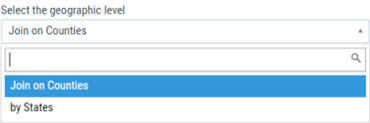
Visibility Slider:
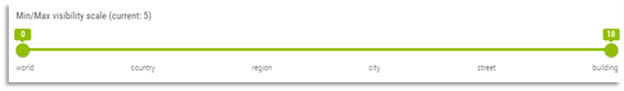
The visibility slider allow to select the visibility range of the current mapping.
|
Example: Let’s say we our data is represented at two levels: a layer US States and a layer US Counties. US States can be visible from world to country and US Counties from country to building. This way, when the map is unzoomed to the whole country, the states are visible and zooming on a state will show the counties. |
Projection on layer
The current mapping can be projected on a geographic layer.

For example, let’s say we have a dataset with some stores in the US represented as points on the map. The dataset can be projected on the US States layer and the result is a polygon layer representing the states and where each indicator come from the stores but aggregated for each state.
This allow to quickly define a spatial hierarchy with the data.
The multi-mapping is also defined from the mapping tab.
The multi-mapping is a powerful feature though it might be difficult to understand. In few words, it allows to define multiple representation types (mappers) on the same dataset.
|
Let’s illustrate with an example: The dataset is a list of stores, each record contains the X/Y coordinates of the stores, a set of indicators (revenue, etc …) and the name the attached to warehouse name. From that dataset, we can define 3 mappers:
In this example, starting from a single dataset, we quickly get a rich map showing thematic layers on the individual stores, their attached warehouse location and the repartition through the regions. |
Once various mappings are defined on a dataset, the thematic wizard will propose the list of available mappings:
The geo-links allow the association of customized link to a geographical dataset in order to query a report, an external application, or to launch a processing from a geographical selection on the map.
The geo-link are accessible complementary to the standard georeports from the info view, from a selection or in the territory management extension.
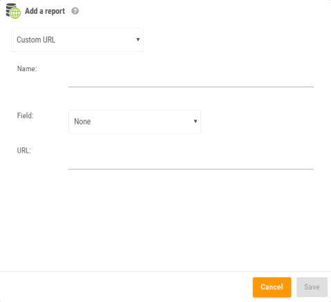
The creation of a geo-link requires 3 pieces of information:
Name: this is the name that will be displayed on the link
Field: the field of the geographical layer which values are sent to the geo-link URL
URL: a URL that can contain the element [values]. At runtime, [values] is replaced by the value of the “field” for the selected object. If several objects are selected, then [values] becomes a list of values separated by comma.
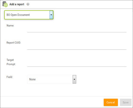
BO Open Document is used to open another BO report from the map. The geographical selection will load automatically the prompt that was defined. The other prompts of the WebI document will be sent as well to the target report.
To add this type of report the following parameters are necessary:
Name: The name that will be displayed in the info window and in the selection tool
Report CUID: The WebI document CUID that was got by right clicking and going to the WebI document properties
Target prompt: The prompt name that was defined in the target report
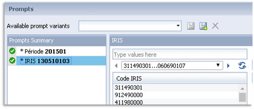
The prompt name will be "IRIS" in this example.
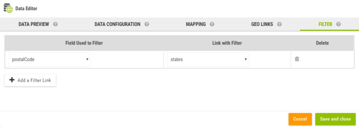
When a map contains one or several filters, it is possible to apply a filter on a geographical layer added and known uniquely by the viewer. This regards the geographical layers resulted from spatial queries or from imported files in the viewer, as well as GIS layers as operational layers.
This implies to have a common attribute with identical values between the filters and dht geographical layer to be filtered.
In order to attach a filter to a dataset, one has to go to the tab FILTER from the Data Editor and enter two values:
The name of the dataset field that will serve as filter
The name of the filter to use of which the selected values will serve the filtering


